ODE(p): Explicit Runge-Kutta methods of arbitrary user-defined order

ODE(p) is a Matlab code that provides Butcher tableaus of explicit (and implicit) Runge-Kutta methods of arbitrary user-defined order.

Construction of high order Runge-Kutta methods in ODE(p)

Once Runge-Kutta methods are discussed in class many students search the web to find a Butcher tableau of the highest order explicit Runge-Kutta method that was revealed so far. They may end up with Hairer's DOPRI(8,5) method. However, it is well-known that implicit ODE solvers can be simply constructed by using the collocation principle. One only needs a quadrature rule for an interval. Once an implicit solver of the requested order is obtained one can change it into an explicit scheme by applying Banach's fixed point method to it.

In the code below we use the Gauss-Legendre quadrature rule. This gives an order of accuracy of p=2*s+1 for s stages. In order to not destroy this accuracy when solving the implicit scheme with Banach's fixed point method one just needs to apply the sufficient number of 2*s fixed point iterations. We call such a scheme GB(p) for 'Gauss-Banach of order p'. ( We actually choose p and then set s=floor(p/2). )

Outline: The code below provides parametric Runge-Kutta methods which for a user-defined parameter s yield an order of accuracy of p=2*s+1 and require 4*s*s evaluations of the flux function. Notice that this concept is already well-known in the literature and is described, e.g., in Hairer, Wanner and Norsett, Solving Ordinary Differential Equations I: Nonstiff Problems, 2nd reviesed Edition, Springer 2009.

Download: ODEp_pack.zip

Observations

First we investigate what the stability regions for large orders look like. Fig.1 shows the stability regions of the explicit Runge-Kutta methods GB(p) for p=3, 6, 9, ... 30. We see that for larger values of p the stability regions look like semicircles with a radius that grows linearly in p. Since the number of flux evaluations (i.e. stages) grows superlinearly with p we can conclude that it is not beneficial to choose p larger in order to perform larger time-steps for stiff problems.
Stability regions of the GB(p) method for p=3, 6,..., 30
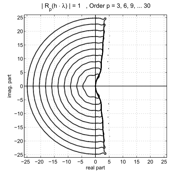
Figure 1: Stablity regions in the complex plane for the explicit
Runge-Kutta methods GB(p) for p=3 to p=30.

We go more into detail for the specific method GB(5). Fig.2 shows again in black the border of the stability region and in the background it shows in colors the magnitude of the stability function. One can observe that in the first and fouth octant there are two regions where the stability function has a value smaller than one. Consequently, the stability regions are in general not simply connected.
Stability region and stability function of GB(5).
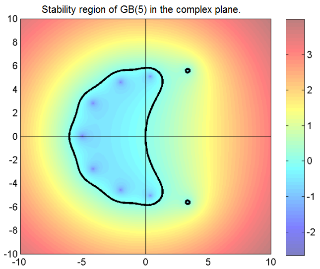
Figure 2: Stability function and stability region of the
explicit Runge-Kutta scheme GB(5) in the complex plane.

Finally we test on the Dahlquist problem { dx/dt = -1*x , x(0)=1 } whether the GB(p) methods converge of order p. Fig.3 lays out the global error of the numerical solutions at time t=1 of the GB methods compared to the analytic solution with dependence on the stepsize h. The slopes of the graphs indicate that the methods GB(p) do indeed converge at least of order p.
Experimental validation of the order of accuracy for GB(p).
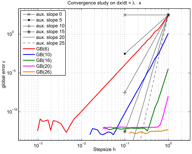
Figure 3: Convergence behaviour of several GB(p) variants
with repect to the time-step.


back to main page: Back