Silver bullet: An optimal control solver
Silver bullet is a
direct transcription finite element method for the numerical solution of one-dimensional
optimal control problems. Instead of collocation it uses L2 plenalties.
While it is trivial to construct examples for which collocation methods
diverge in general, the L2 penalty approach is proven to be convergent
for the general one-dimensional optimal control problem with general
differential-algebraic equality- and inequality-constraints. While the
code is under progress, I present on this page some numerical results.
Origins of the method
In 2016/2017 I had an employment at the Mercedes Formula One team.
All Formula One teams use numerical methods for optimal control to
minimize lap time. I was working on a replacement for the current
numerical optimization methods. Working on these methods during my
employment raised my interest for research in new numerical methods for industrial
optimal control problems.
Practical methods discretise the optimal
control problem in a direct way into a large sparse nonlinear program. This in turn is solved using
software for constrained nonlinear optimization. The process of transcription
from an infinite-dimensional optimisation problem into a
finite-dimensional one involves numerical approximation schemes
for the underlying differential-algebraic constraints. During the time
of my employment, there was no method known that had a
theoretical proof that the numerical solution
would converge to the analytic solution of the original problem. This
is why after my employment and completion of my master's degree I
performed research to finally develop a transcription method that is
proven to be convergent.
The method is described here: https://arxiv.org/abs/1712.07761
. Dr Eric Kerrigan from Imperial College London and I wrote a paper
that presents a very thorough proof of convergence for this method: https://arxiv.org/abs/1810.04059 . The proof works under very mild assumptions.
The
idea of the method is as follows. As common, finite elements are used
to parametrise the arcs of the solution. Since
collocation can diverge, the
path-constraints are treated not with collocation but by
integrating their Lebesgue two-norm and adding it as a quadratic
penalty to the cost-functional.
Inequality constraints are treated with an integral of a
logarithmic barrier function that is also added to the
cost-functional. The L2 penalty
yields symmetric stencils and is apparently stiffly stable. In result
of the constraint treatments on the continuous level we obtain a
finite-dimensional unconstrained penalty-barrier nonlinear programming
problem. This is solved efficiently with an SQP-like numerical
optimization method. The arising linear systems have narrow-banded
matrices and can be solved fully in parallel, employing a
divide-and-conquer technique.
Examples
John Betts provides a collection of optimal control problems. Below we
solve a small selection of problems described therein, using our
method. All problems were solved with isotropic mesh, finite elements
of polynomial degree 4 to 10, and all in less than 5 minutes.
The
computations were performed without parallelism in Matlab 2016b on a Lenovo Yoga from
2015 with Intel i7 4800U processor and 8GB RAM. Since our method
does not need to distinguish between states and controls, so do we not
either, and call everything "species". The dimensions of the problems
are between 1000 and 8000 degrees of freedom for the non-linear
program. We plan for a parallel implementation in C++ for a compute cluster. In future we want to solve far bigger problems.
Aly-Chan problem
This problem has four smooth species. u is a fully singular arc
that touches its box-constraints [-1,1] only at one time-instance.
Numerically this problem is difficult to treat as usually the NLP
solver does not know what use to make of the degrees of freedom in u
and thus starts ringing wildly. In our case we find that the numerical
solution is a smooth approximation to the analytic solution, which is
u(t)=-sin(t).
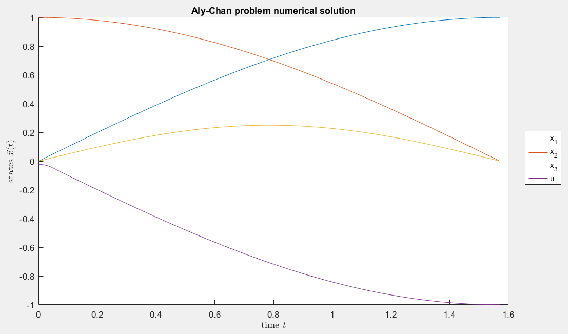
Figure 1: Numerical solution to the Aly-Chan problem.
Brachistochrone problem
The problem consists of four smooth species. The problem is
well-scaled. The solution can be rapidly approximated with a few
elements of high order. A difficulty with this problem is that the
end-time is the variable to minimize. After transforming the system
into an interval of fixed length, the constraint equations are
nonlinear of type res=x1 * x2 * cos(x3). Our NLP solver requires about
40 iterations, depending on mesh-size and elemental degree.
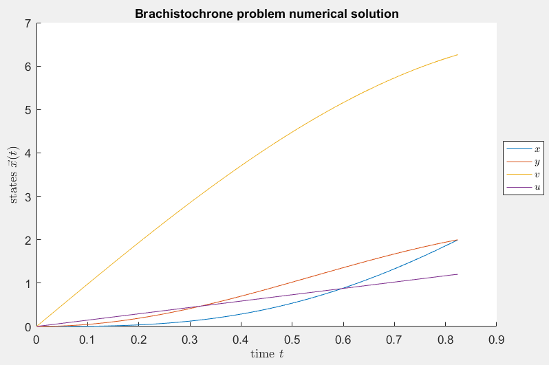
Figure 2: Numerical solution to the brachistochrone problem.
Chemotherapy
This is a badly scaled non-linear problem of five smooth
species. It stems from a biological model for the computation of a
treatment plan for HIV with chemotherapy.
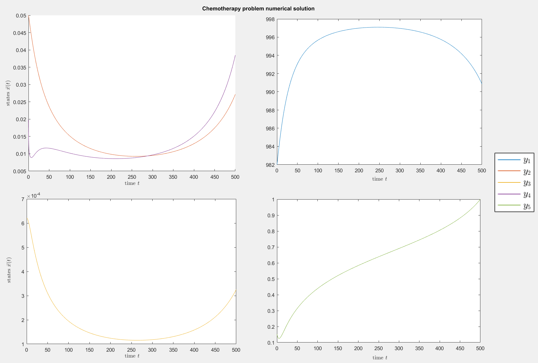
Figure 3: Numerical solution to the chemotherapy problem.
Container crane problem
This is a problem with 8 smooth species. We have no deep
understanding of this problem, yet, but were able to verify through
mesh convergence that the presented arcs give an accurate solution.
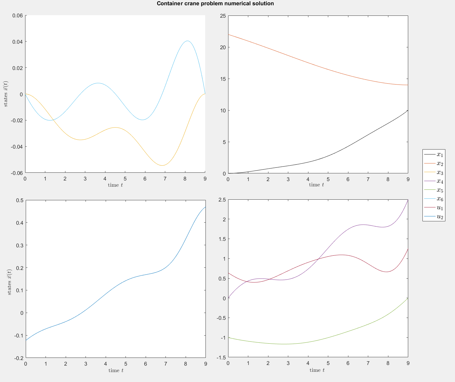
Figure 4: Numerical solution to the container crane problem.
Drug treatment problem
This is a badly scaled problem of four smooth species that arises
from a biological model for a drug treatment of HIV. While smooth,
three of the four species have non-smooth first derivatives, making it
difficult for the finite elements to accurately represent the exact
solution.
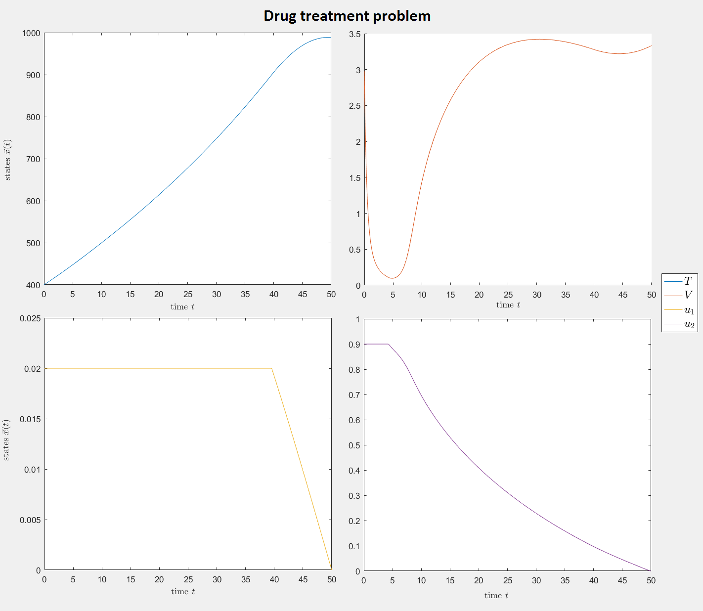
Figure 5: Numerical solution to the drug treatment problem.
Free flying robot problem
This problem has twelve species with bang-bang controls. We
used 80 finite elements of degree 8. Six out of the twelve states are
non-smooth. While the arcs of the smooth species are well represented
by the numerical solution, we find some non-optimal mesh-related
artifacts nearby the discontinuities. This is because the high
polynomial degree does not help approximating discontinuities well on a
coarse mesh.
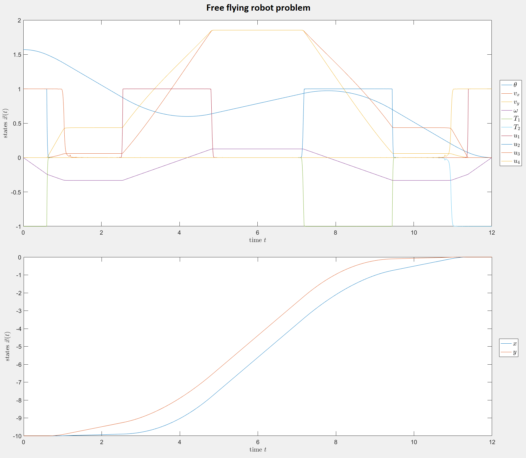
Figure 6: Numerical solution of the free flying robot problem.
The free flying robot problem searches for an economic control to
reposition a robot in space. The robot has pneumatic propulsions.
The amount of used pressure gas is minimized. The animation below
visualizes the above control diagram.
Figure 7: Animation of the optimal dynamics for the free flying robot.
An example from raceline optimization
The following is a crude testing model for computing
time-optimal trajectories through a track. The objective is to minimize
the end-time. There are no-slip path-constraints, initial velocity constraints
(start at rest), and start and finish coordinate constraints along the path of the track.
The optimal arcs to be found involve raceline (plotted in blue), and
arcs of accelerations and velocities.
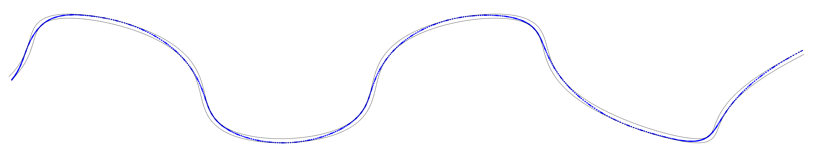
Figure 8: Raceline along sample track.
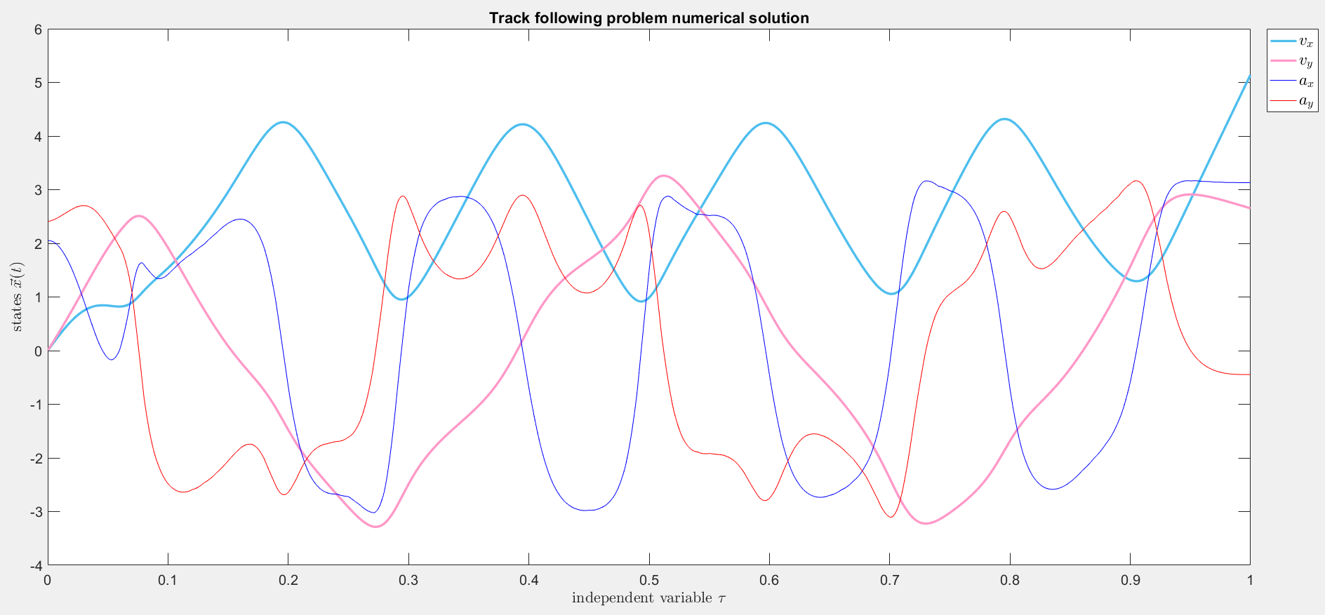
Figure 9: Optimal velocities and accelerations along raceline.
The problem statement below consists of three parts: Equations (2)-(5)
model the track parametrization. T is final time, s is track
parametrization, n is track tangential vector (solved as part of the
control problem), lambda is an auxiliary to express the tangent
condition of n to the track. gamma is a given curve that returns track
center line coordinates with respect to input s of track
parametrization. Equations (6)-(8) model the dynamics. Equations
(9)-(11) form the actual car model. Equations (12)-(14) form the point
constraints. (12)-(13) make sure that the car drives from the start
line to the finish line on the track. (14) gives the initial velocity
vector. The model is simple and does not consider, e.g., angular
orientation of the car. Constraints in (15) involve the track width B
and the square of the maximum acceleration u^2_max .
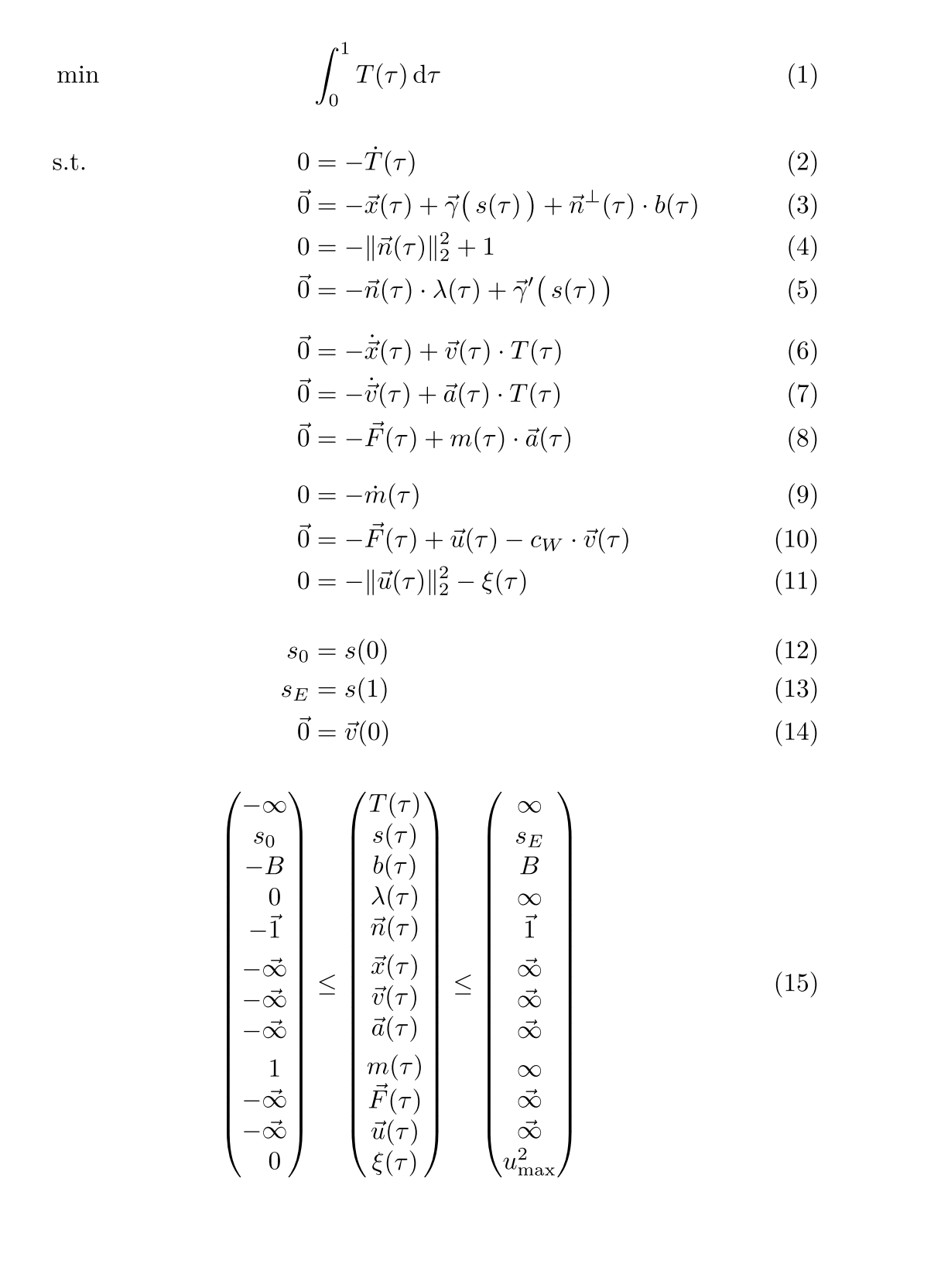
Figure 10: Problem statement for raceline optimization with a simplified car model.
Contact via e-mail: MartinNeuenhofen@googlemail.com