Some Numerical Applications from Computational Engineering
On this page I present algorithms for solving some frequently used mathematical models.
The intention is to give an overview of applications for numerical mathematics.
Partial differential equations
Partial differential equations are used to model physical phenomena in
materials, such as gases, liquids and solids. For instance, the motion
of water, the expansion of gases, the dynamics of heat, and elastic as
well as non-elastic deformations can be described using these kind of
equations.
Poisson's equation
The Problem
Poisson's equation counts as the test problem for linear elliptic
partial differential equations. It occurs in many phyical models. For
instance the stationary temperature distribution in solid
heat-conductive materials subject to local heating or cooling as well
as the
stationary elastic deformation of membranes under load can be predicted
to a certain extend by a physical model that employs a Poisson equation.
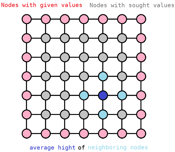
Here we look into the homogeneous Dirichlet boundary-value Poisson problem in two dimensions. My Bachelor's thesis described this problem in mathematical terms, whereas here a plastical presentation is followed in Figure 1.
Plastically speaking, the problems asks to compute the shape of a hill
of which each point is on
the average hight of its neighbouring points. The figure illustrates
this with dots on a grid. Each dot must have a value. In the Dirichtlet
problem, values on the pink dots are prescribed. Then, the mathematical
task is to find suitable values for all the grey dots such that each
dot has the average value of its four neighbours. For instance, the
dark-blue node shall have the average value of the four light-blue
nodes. There is exactly one unique solution such that every grey dot
has the average value of its neighbors.
Figure 1: Grid lines and nodes of a Cartesian grid for
the numerical solution of a Poisson problem.
Temperature distributions in metals follow a principle like this, in
that the local temperature in a material takes on the average value of
the temperatures in the materials that surround it. Therefore, solving
Poisson's equation can have practical relevance for predicting the heat
distribution and thereby possibly affected material properties (such as
stability or deformation).
In the following, we present a way for computing a solution values for all the grey dots, using the help of a digital computer.
In order to find an accurate solution, the grid should be desirably
fine. The above figure shows a 7x7 grid. For more realistic
representations, grids with 1000x1000 points or beyond are used. Then,
the number of
sought values for the grey dots is in the order of millions. This large
number raises the question
of how to compute the solutions in an
acceptable amount of time. One naive way to find a solution for all
nodes works by repeated averaging: Going repeatedly from upper
left to lower right, each point is set to the average of its four
neighbouring points. This is called Jacobi's method. To get acceptable
results with Jacobi's method, the computation time increases by a
factor of 2^4 = 16 when increasing the number of grid lines in both
directions by the factor 2. One says Jacobi's method has complexity
order 4.
The Solver
More efficient methods try to find lower complexity orders. The best
possible order is 2, and one can realize it by switching with Jacobi's
method on different grid sizes. This is called a multi-grid method. The
following Matlab code gives a simple implementation of a V-cyclic
multi-grid method.
The solver initializes a matrix U with values of the numerical
solutions for each grid point. The border values of matrix U have to be
written to the Dirichlet boundary values. For the Smooth-function
Jacobi's method was chosen.
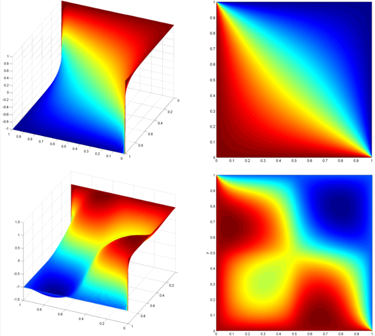
The following pictures show sample solutions of the multi-grid solver
on 2049x2049 grid points after seven iterations. The pictures show
sample solutions for the homogeneous and an inhomogeneous case for the
same boundary conditions.
Figure 2: Visualisation of two solutions of Poisson's equation with Dirichtlet boundary conditions.
Incompressible Navier-Stokes-equations
The Problem
These equations are widely known as the fundamental equations for modelling
the dynamics of fluids. Although the derivation of these equations and
particularly of the friction term are complicated, their meaning is
arguably simple.
One can imagine flow as a vector field. Each arrow direction gives
the local flow direction and its length denotes the local velocity. As
for Poisson's equation we consider a region in which we want to predict
the flow mathematically. When looking at the vector field, which describes the flow in
one moment, the Navier-Stokes equations tell on the basis of the current flow how it will change in the next moment. To make it
precise, it exactly tells the following:
The local flow moves in its
own direction. This means in each local region the arrows move with
their velecity and direction. This models the momentum transport.
Simultaneously, neighbouring arrows assimilate to each other. This models the inner friction of the fluid.
One term that is missing yet in the imagination is the pressure term.
One can imagine that each group of eight directly neighbored nodes
defines a small cube. For each cube there is a pressure value. When
setting the pressure in one clube high while not changing the pressure
value values in the surrounding cubes, then fluid is pushed out of this
cube, which means the arrows of the nodes of the vertices of the cube
will point more apart from each other. The clue is now to find pressure
values for all the cubes such that in each moment in- and outflow
for each cube cancel to zero. This last rule models local conservation of fluid volume.
The Solver
One way for numerical computation of such vector fields is to update
the vector field according to the rules of momentum transport and
friction with a so-called ODE-integrator (ODE stands for 'ordinary
differential equation', cf. below) and then computing values for the
pressures in the cubes, such that the fluid volume is conserved.
When doing so, one has to mind several numerical difficulties:
The arrows may begin to oscillate and the underlying numbes
produce meaningless results. This is indicated by the momentum
transport. To overcome this, the friction must be large enough
(advection needs minimal numerical diffusion) and the time step has to
be small enough (CFL condition).
To find numerical values for the pressure, one
would have to compute a linear least-squares solution to a singular
linear regression problem. The correction of the
vector field can then be computed by the residual of this least-squares
solution. When solving the least squares problem via the normal
equation one obtains a Poisson problem for the pressure. This can by
solved most efficiently with the multi-grid method from above or a
preconditioned Krylov subspace method.
The following Matlab program can be used to compute flows in two spatial dimensions around
hand-drawn objects. You draw a black-white-picture, save it
as PNG or JPEG, right click it in the Matlab window, transform it into
a tensor and give this tensor as only input argument to the Usecase
function. The function computes and visualizes the flow around the black shape
after specific time steps. The visualization produces JPEG images
after each few time steps. The function Streamplotter can
be used with the outcome of Usecase to visualise the stream lines.
The pixels of the hand-drawn image accord to the two dimensional cubes of the
numerical grid. To get a feeling on how long your computer needs to
compute a solution, you are recommended to start with small pictures,
e.g. 200 by 200 pixels.
The solution is obtained by a Lax-Friedrich-scheme for the advection
and diffusion operator and a direct solver on the Tikhonov-regularized
normal equation for the pressure. This was found to need less time then
iterative solution for grids up to 800 by 600 cells. For larger grids
one can also enable iterative solution over IC(T)-precondtioned
CG-method. PCG was preferred over Multigrid because PCG's convergence seems less dependend on the shape of the obstacle.
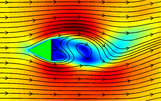
Fig. 3 visualizes the instationary flow around a
triangular shape (marked in green).
The logo on the main page of my homepage is also computed with this
program.
Figure 3: Stream lines of the instationary 2D flow of an
incompressible viscous fluid around a triangular shape.
Transport of scalar field in fluids
For many applications it is necessary to compute the transport
of a solute in a fluid; for example when modeling the diffusion of
a poisson gas in a metropolitan area or the motion of cigarette smoke
throw the air. When dealing with such advective and diffusive passive
matters, one can simulate the distribution of the respective property
over time and space with finite volumes: The finite volumes fill the
simulation area. For each finite volume we take an integral of how much
matter flows in and out. To give a computational example, the
Navier-Stokes-solver from above was extended by a transport equation of
a passive scalar field.
The Solver computes the motion of smoke lines around a nozzle as
shown in Fig. 4. Input arguments, geometries and
boundary conditions are optional.
Figure 4: Animation of the stream flow through a nozzle.
Ordinary differential equations
Ordinary differential equations put the change of a property over time
in correlation to the property itself. One example is radioactive
decay: The magnitude of decay of a substance is proportional to its
amount. The solution of such a differential equation is an exponential
function. In the following there are examples of applications with
ordinary differential equations.
Simulation of frameworks
One might know the computer game bridge builder. In this game the player has to
design a bridge framework in two dimensions that satisfies certain
stability conditions. This game bases on a model: A bridge consists of
nodes and bars. The nodes are points in which at least two bars are
connected. The geometry of the bridge can be defined by the x- and
y-coordinates of the nodes and a table that lists, which nodes are
connected to each other by a bar. As the bridge deforms under
gravitational and other optional outer forces, those nodes, which are
not connected to the foundation of the bridge, change their coordinates;
they change their position. They move, so they have a velocity. This
affects the length of the bars. As the bars get stretched and
compressed they act forces on the nodes, which are parallel to the
bars direction and of which the magnitude increases with the change in
length. For each node these forces can be added vectorial to a
resultant force. This force defines how the velocities of the nodes
change with time (Newtons third law). As a conclusion, the temporal change
of the positions of the nodes is a function of the positions of the
nodes. By linearisation of these temporal changes over small time
intervals one obtains an approximation of the whole framework's motion.
The simulation cycle now looks the following:
Initialization:
Define positions of all nodes.
Define bar connections between the nodes.
Compute the length of all bars (Pythagoras).
The velocities v of all nodes are set to zero.
Compute resultand forces on each node.
Compute deformation of all bars.
Compute of the reactant forces of the bars.
Add outer forces as graviational forces on the nodes.
Sum up all forces on each node to a resultant force.
Compute a time step (here: explicit Euler's method).
Define a value for a very small time intervall and call it dt .
Devide the resultant force of each node by its weight. The result is called "acceleration", symbol a .
The acceleration overwrites the velocity of each node: v := v + dt * a .
The velocity of each node overwrites its position vector x in the following way: x := x + dt * v .
Close the loop: Plot the framework and go back to step 2.
The above Matlab code simulates the dynamics of frameworks. For
the reactant forces of the bars it uses Hook's model (reactant force is
assumed to be proportional to the deformation). The file Geometries contains a set of examplary geometries. Fig.5 shows animations for a zig-zag
geometry which is used as a bridge (left) and as an arm (right).
Figure 5: Simulation of the dynamic deformation of one idealized framework for different anker nodes.